Hybrid Genetic Search meta-heuristic example

The meta-heuristic used is vidalt/HGS-CVRP: Modern implementation of the hybrid genetic search (HGS) algorithm specialized to the capacitated vehicle routing problem (CVRP). This code also includes an additional neighborhood called SWAP*.

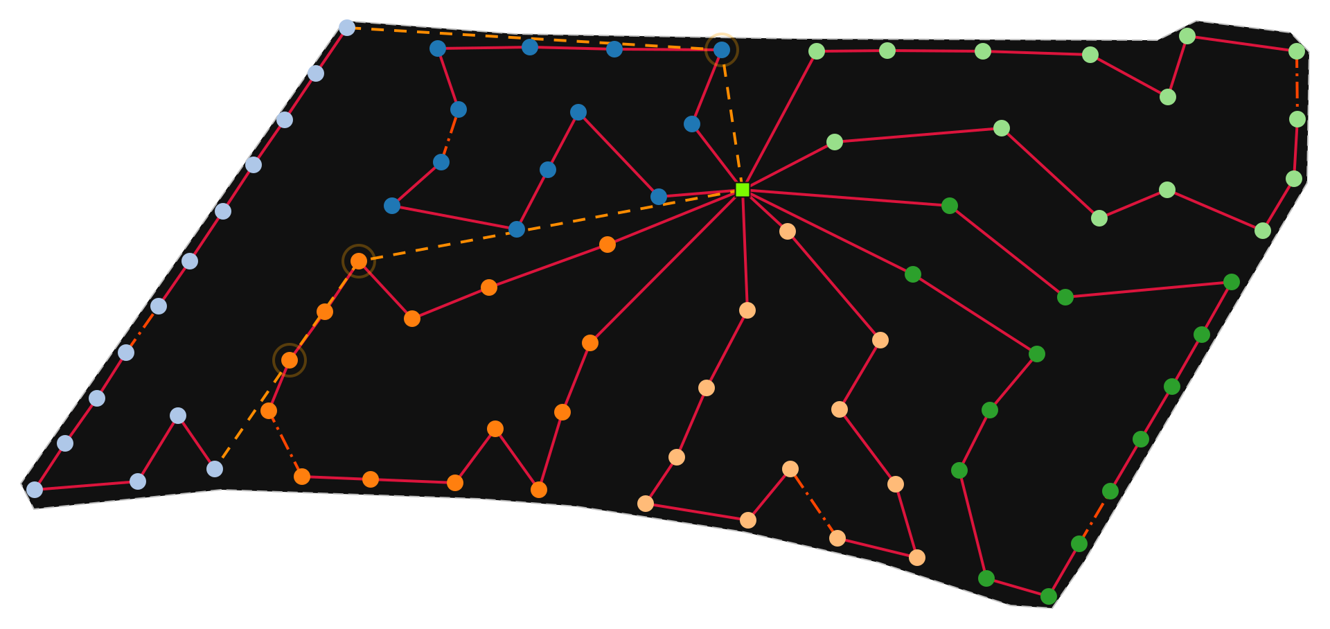
HGS-CVRP can produce both radial and ringed topologies. By default, it solves an Open-CVRP yielding a radial topology. With ringed=True, it solves a closed CVRP where every route returns to the depot, producing a ringed topology.

Solutions produced by this method can be used directly or as warm-starts for MILP models.

If a routeset is desired, use PathFinder.

from optiwindnet.importer import load_repository
from optiwindnet.svg import svgplot
from optiwindnet.baselines.hgs import hgs_cvrp
from optiwindnet.mesh import make_planar_embedding
from optiwindnet.pathfinding import PathFinder
from optiwindnet.interarraylib import G_from_S, as_normalized

Load Hornsea

locations = load_repository()

L = locations.hornsea
svgplot(L)

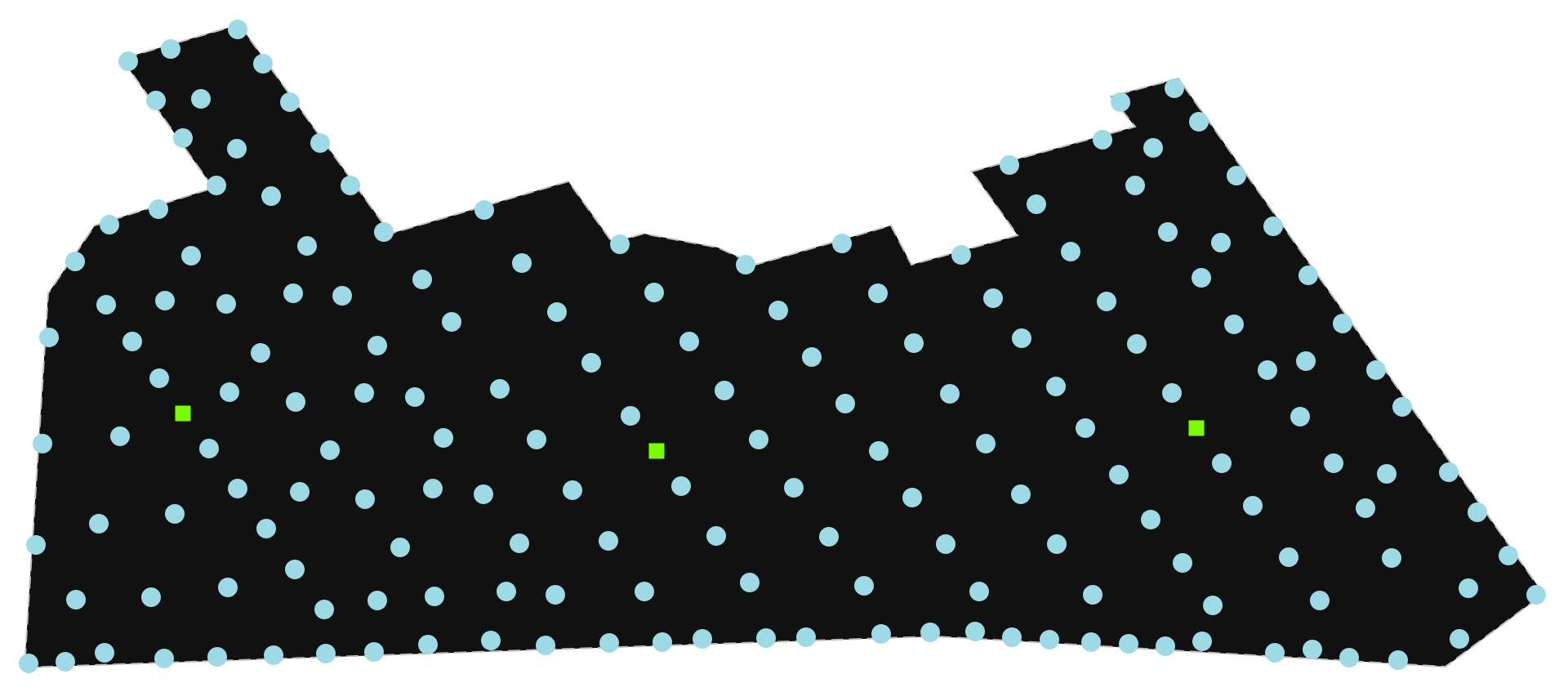
Optimize Hornsea

P, A = make_planar_embedding(L)
S = hgs_cvrp(as_normalized(A), capacity=7, time_limit=0.5)
print(S.graph['solution_time'])
G = G_from_S(S, A)
svgplot(G)

(0.13, 0.1, 0.28)

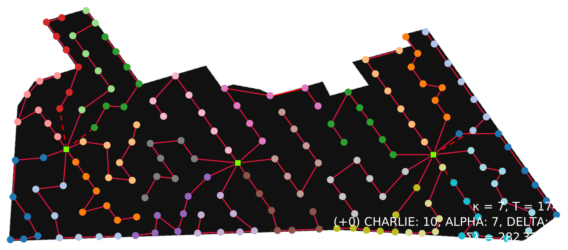
Route the feeders so as to avoid crossings

H = PathFinder(G, P, A).create_detours()
svgplot(H)

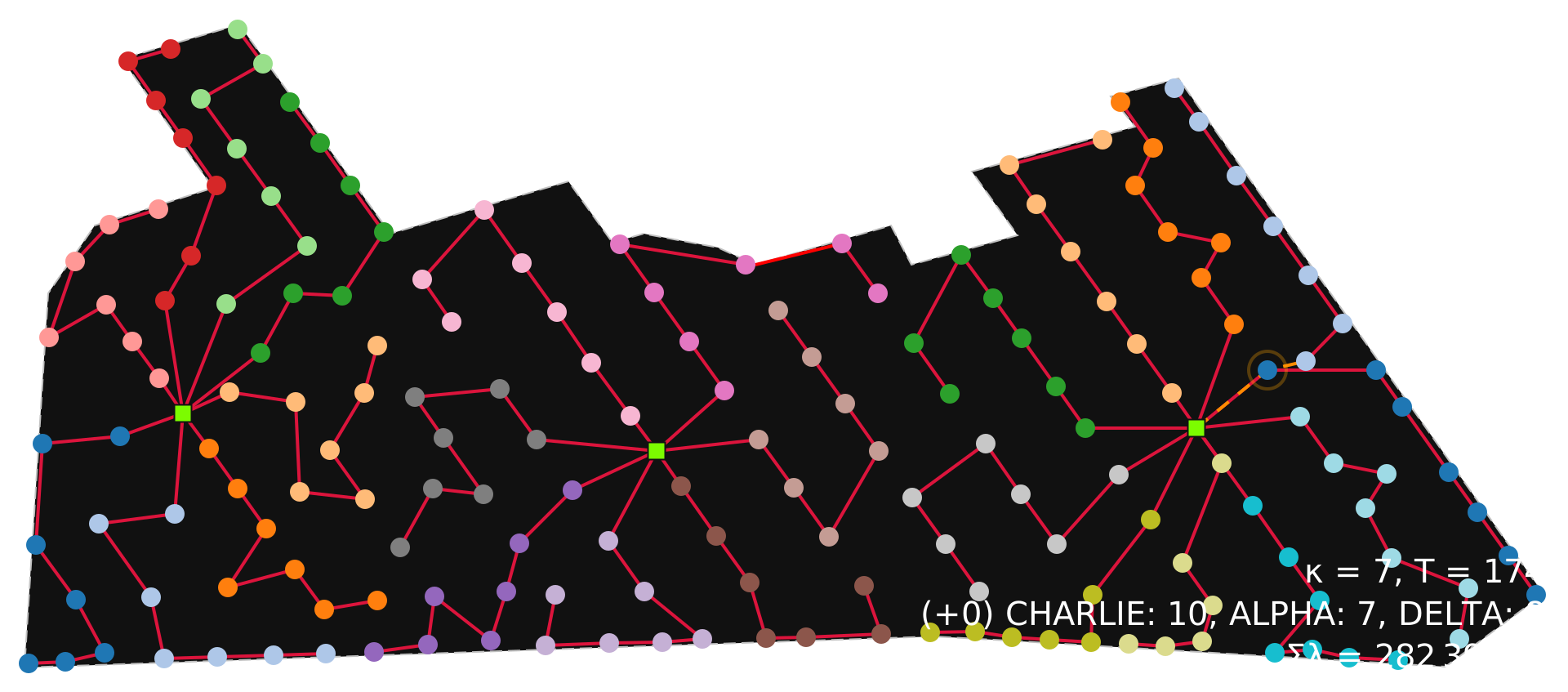
Check the HGS-CVRP log

There are two alternatives to see the HGS log:

1. Store it in the solution object (must wait until HGS has finished)

2. Stream it using a callback function that gets one line per call

L = locations.meerwind
P, A = make_planar_embedding(L)

Store the log

S = hgs_cvrp(
    as_normalized(A),
    capacity=7,
    time_limit=0.5,
    keep_log=True,
)

print(S.graph['method_log'])

----- FLEET SIZE WAS NOT SPECIFIED: DEFAULT INITIALIZATION TO 18 VEHICLES
----- INSTANCE SUCCESSFULLY LOADED WITH 80 CLIENTS AND 18 VEHICLES
----- BUILDING INITIAL POPULATION
----- STARTING GENETIC ALGORITHM
It      0      2 | T(s) 0.05 | Feas 60 11.17 11.33 | NO-INFEASIBLE | Div 0.45 -1.00 | Feas 1.00 1.00 | Pen 5.81 0.85
It    500    122 | T(s) 0.19 | Feas 27 11.02 11.14 | NO-INFEASIBLE | Div 0.45 -1.00 | Feas 1.00 1.00 | Pen 2.58 0.38
It   1000    410 | T(s) 0.34 | Feas 35 11.02 11.11 | NO-INFEASIBLE | Div 0.41 -1.00 | Feas 1.00 1.00 | Pen 1.14 0.17
It   1500    910 | T(s) 0.50 | Feas 43 11.02 11.10 | Inf 1 11.91 11.91 | Div 0.38 -nan | Feas 0.99 1.00 | Pen 0.51 0.10
----- GENETIC ALGORITHM FINISHED AFTER 1509 ITERATIONS. TIME SPENT: 0.500349

Stream the log

S = hgs_cvrp(
    as_normalized(A),
    capacity=7,
    time_limit=0.5,
    log_callback=(lambda line: print(line, end='')),
)

----- FLEET SIZE WAS NOT SPECIFIED: DEFAULT INITIALIZATION TO 18 VEHICLES
----- INSTANCE SUCCESSFULLY LOADED WITH 80 CLIENTS AND 18 VEHICLES
----- BUILDING INITIAL POPULATION
----- STARTING GENETIC ALGORITHM
It      0      2 | T(s) 0.05 | Feas 60 11.26 11.37 | NO-INFEASIBLE | Div 0.45 -1.00 | Feas 1.00 1.00 | Pen 5.81 0.85
It    500    281 | T(s) 0.19 | Feas 27 11.04 11.15 | NO-INFEASIBLE | Div 0.43 -1.00 | Feas 1.00 1.00 | Pen 2.58 0.38
It   1000    282 | T(s) 0.34 | Feas 35 11.02 11.11 | NO-INFEASIBLE | Div 0.39 -1.00 | Feas 1.00 1.00 | Pen 1.14 0.17
It   1500    782 | T(s) 0.50 | Feas 41 11.02 11.13 | Inf 4 11.51 11.78 | Div 0.39 0.38 | Feas 0.96 1.00 | Pen 0.51 0.10
----- GENETIC ALGORITHM FINISHED AFTER 1506 ITERATIONS. TIME SPENT: 0.500381

print(S.graph['solution_time'])
G = G_from_S(S, A)
svgplot(G)

0.34

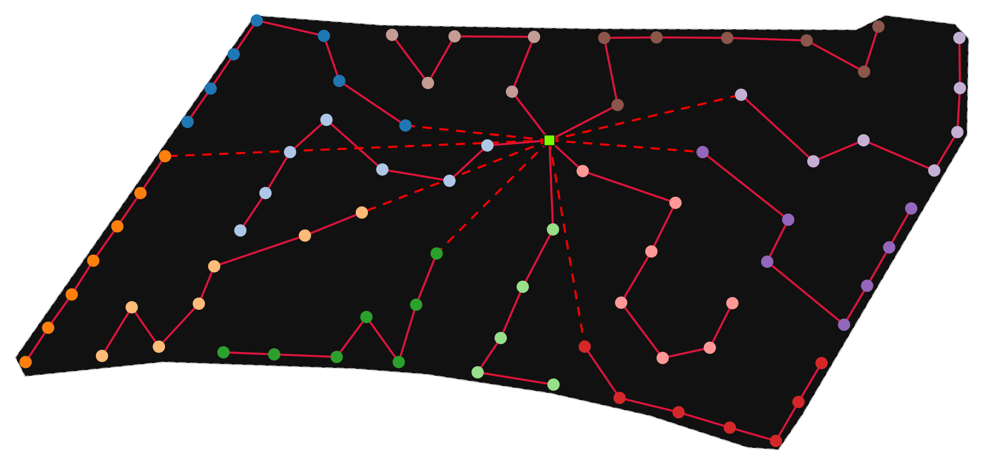
Optimize with Ringed Topology

With ringed=True, HGS-CVRP connects subtrees into closed loops (rings) attached to the substation at both ends.

S_ring = hgs_cvrp(as_normalized(A), capacity=7, time_limit=0.5, ringed=True)
G_ring = G_from_S(S_ring, A)
H_ring = PathFinder(G_ring, P, A).create_detours()
svgplot(H_ring)

Current HGS options

hgs_cvrp() supports multiple substations: it clusters terminals by root and solves each cluster. Use seed for reproducible runs. By default repair=True iteratively repairs crossings; max_retries bounds that work, so total runtime can reach (max_retries + 1) * time_limit.

vehicles is normally an upper bound on feeder count. Set balanced=True to balance feeder loads. vehicles_exact=True fixes the count, but requires balanced=True and is limited to a single-root, non-ringed problem. HGS produces an electrical topology; use G_from_S() and then PathFinder to obtain physical routes.