Note: many of the jupyter notebooks provided here have SVG figures as cell outputs, which will only be displayed by JupyterLab or Jupyter Notebook if the notebook is marked as trusted (In JupyterLab: Ctrl+Shift+C -> Trust Notebook).

Data Input

There are 4 alternatives to import wind farm layout data for use within OptiWindNet:

• Numpy arrays through OptiWindNet API

• windIO YAML file

• .yaml file (OptiWindNet schema)

• .osm.pbf file

from optiwindnet.svg import svgplot

Numpy arrays + OptiWindNet API

from itertools import pairwise
import numpy as np

from optiwindnet.interarraylib import L_from_site

# all coordinates are sequences of (x, y) pairs
# if input coordinates are in arrays X and Y, use `np.hstack((X, Y))`
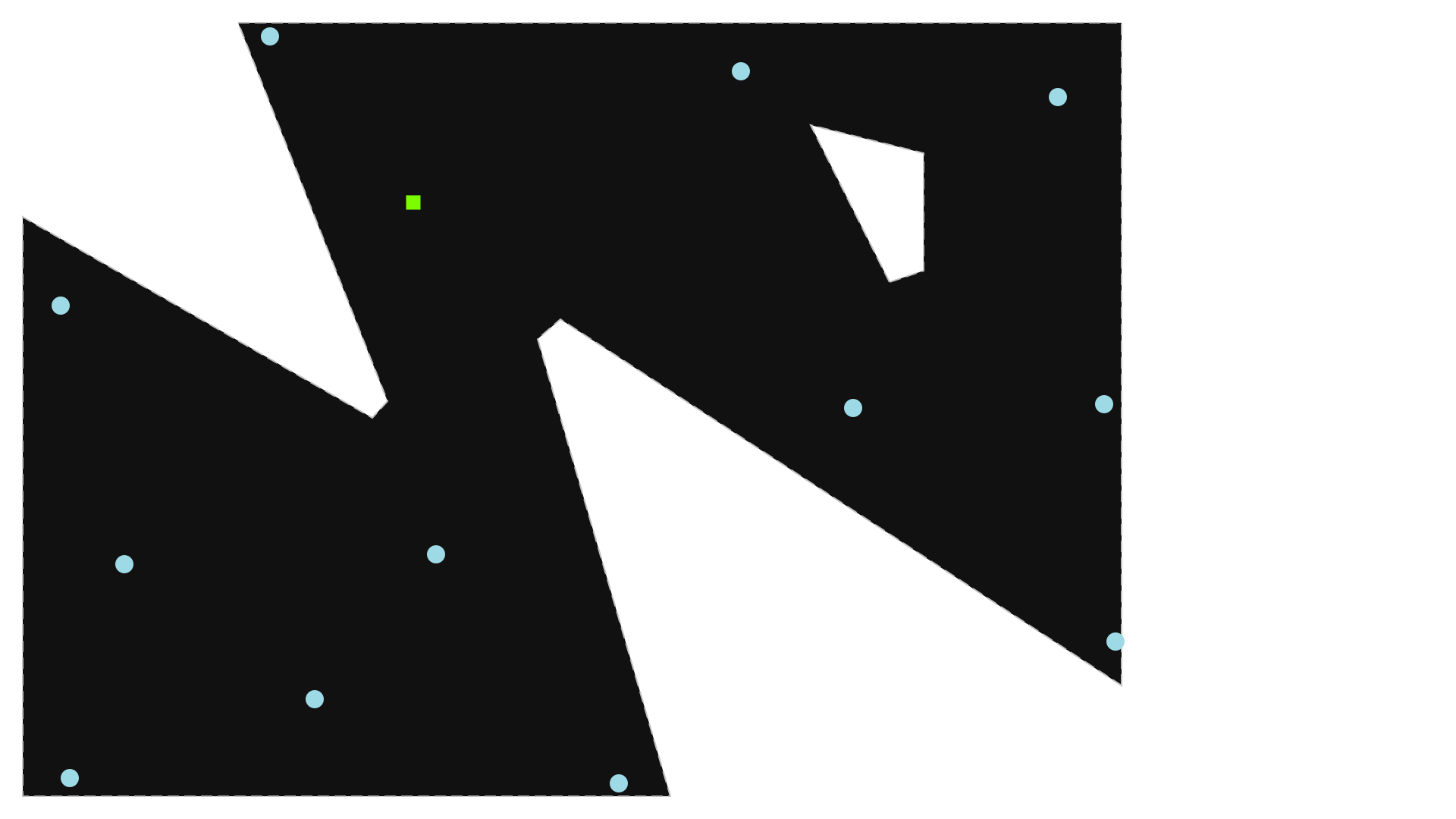
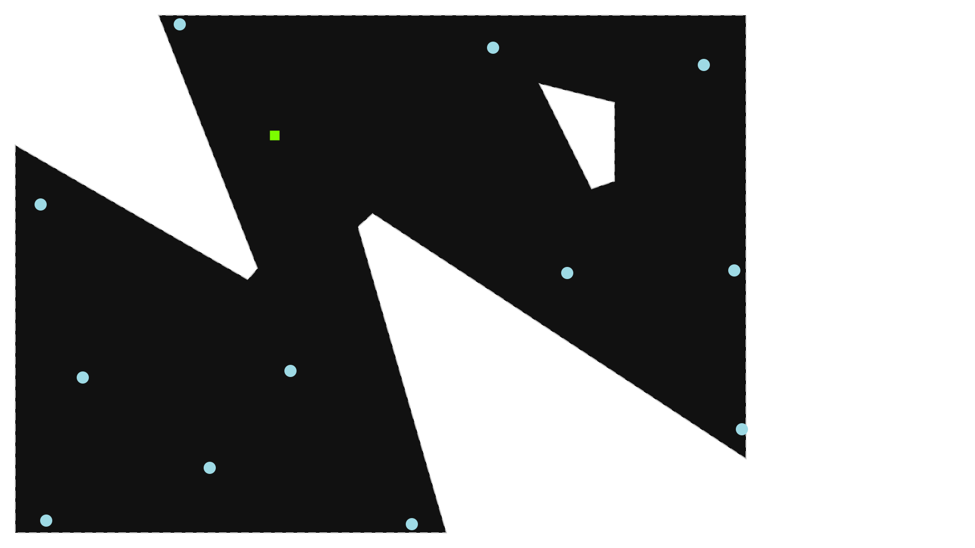
border = np.array( # coordinate sequence defines the polygon, last-first segment implicit
    [[1951, 200], [1951, 1383], [386, 1383], [650, 708], [624, 678],
     [4, 1036], [4, 3], [1152, 3], [917, 819], [957, 854]],
    dtype=float)
# 'obstacles' is an optional location attribute
obstacles = [
    # - obstacles must be strictly inside the border polygon
    # - undefined behavior if obstacles and border overlap
    # first obstacle
    np.array([[1540, 920], [1600, 940], [1600, 1150], [1400, 1200]]),
    # [second obstacle] ...
]
substations = np.array([[696, 1063],], dtype=float)
turbines = np.array(
    [[1940, 279], [1920, 703], [1475, 696], [1839, 1250],
     [1277, 1296], [442, 1359], [737, 435], [1060, 26],
     [522, 176], [87, 35], [184, 417], [71, 878]],
    dtype=float
)
R = substations.shape[0]
T = turbines.shape[0]
border_sizes = np.array([border.shape[0]] +
                        [obstacle.shape[0] for obstacle in obstacles])
B = border_sizes.sum()
obstacle_idxs = np.cumsum(border_sizes) + T

L = L_from_site(
    R=R, T=T, B=B,
    border=np.arange(T, T + border.shape[0]),
    obstacles=[np.arange(a, b) for a, b in pairwise(obstacle_idxs)],
    name='Example Location',
    handle='example',
    VertexC=np.vstack((turbines, border, *obstacles, substations)),
)
svgplot(L)

windIO YAML file

See the windIO documentation for more information on that format.

from optiwindnet.importer import L_from_windIO

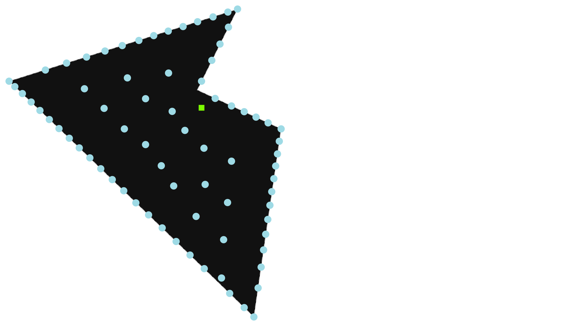
L = L_from_windIO('data/IEA37_Borssele_Irregular_System.yaml')
svgplot(L)

YAML input file

from optiwindnet.importer import L_from_yaml

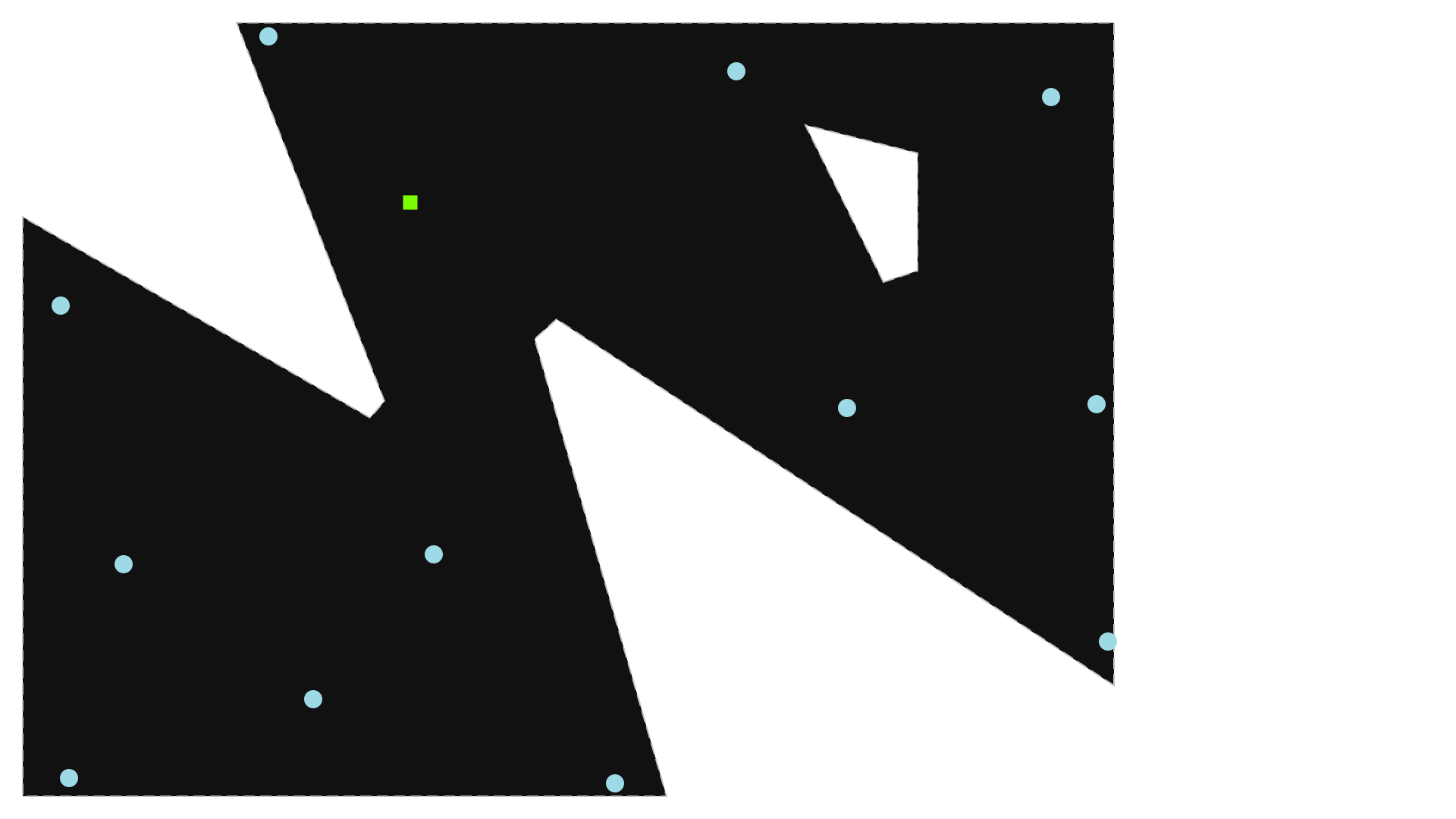
The example YAML file is bundled with the source distribution; this notebook reads it without creating or modifying files.

L = L_from_yaml('data/example_location.yaml')
svgplot(L)

OSM.PBF input file (OpenStreetMap Protobuffer Format)

The JOSM open-source map editor is recommended if using this format: https://josm.openstreetmap.de/. In addition, the JOSM plugin pbf is required to save in the .osm.pbf format. The plugin opendata is useful for importing many common GIS file formats.

The OpenStreetMaps objects used for representing a windfarm location are:

• nodes

• ways

• multipolygons (relation between closed ways)

Wind turbines are represented by nodes with the tag power=generator. Substations are represented either by nodes or by closed ways tagged power=substation or power=transformer. Substations based on ways will be reduced to the point at the centroid of the polygon defined by the way.

The border of the windfarm can be a closed way tagged power=plant. If obstacles are required, then the closed way for the border must be combined with the closed ways for the obstacles in a multipolygon with the tag power=plant (in which case the ways themselves should not be tagged).

See optiwindnet/data/*.osm.pbf for more examples.

from optiwindnet.importer import L_from_pbf

L = L_from_pbf('data/example_location.osm.pbf')
svgplot(L)