🚀 Quick Start

Concepts: Problem · Optimization approaches Advanced API: 🚀 Quick Start

This notebook shows the minimum steps needed to optimize an electrical network for a wind farm with OptiWindNet.

Steps

An OptiWindNet network optimization involves two components:

• A WindFarmNetwork containing the problem data and options.

• A Router defining the algorithm used to solve it.

The network optimization can be performed in the following steps:

1. Create a WindFarmNetwork instance

2. Define a router

3. Run the optimization and get the results

1. Create a WindFarmNetwork instance

The WindFarmNetwork component stores the problem data, invokes its Router during optimization, and stores the resulting topology and routed network. See 📦 WindFarmNetwork for its key methods.

from optiwindnet.api import WindFarmNetwork

Load location data

Note: For details about OptiWindNet’s load_repository(), check 🗂️ Locations.

from optiwindnet.api import load_repository

locations = load_repository()
L = locations.doggerA

Initialize a WindFarmNetwork instance with a prebuilt L and a desired maximum cable capacity (See Data Input for various input formats.)

wfn = WindFarmNetwork(L=L, cables=8)
results = []  # (router, topology, length) of each example

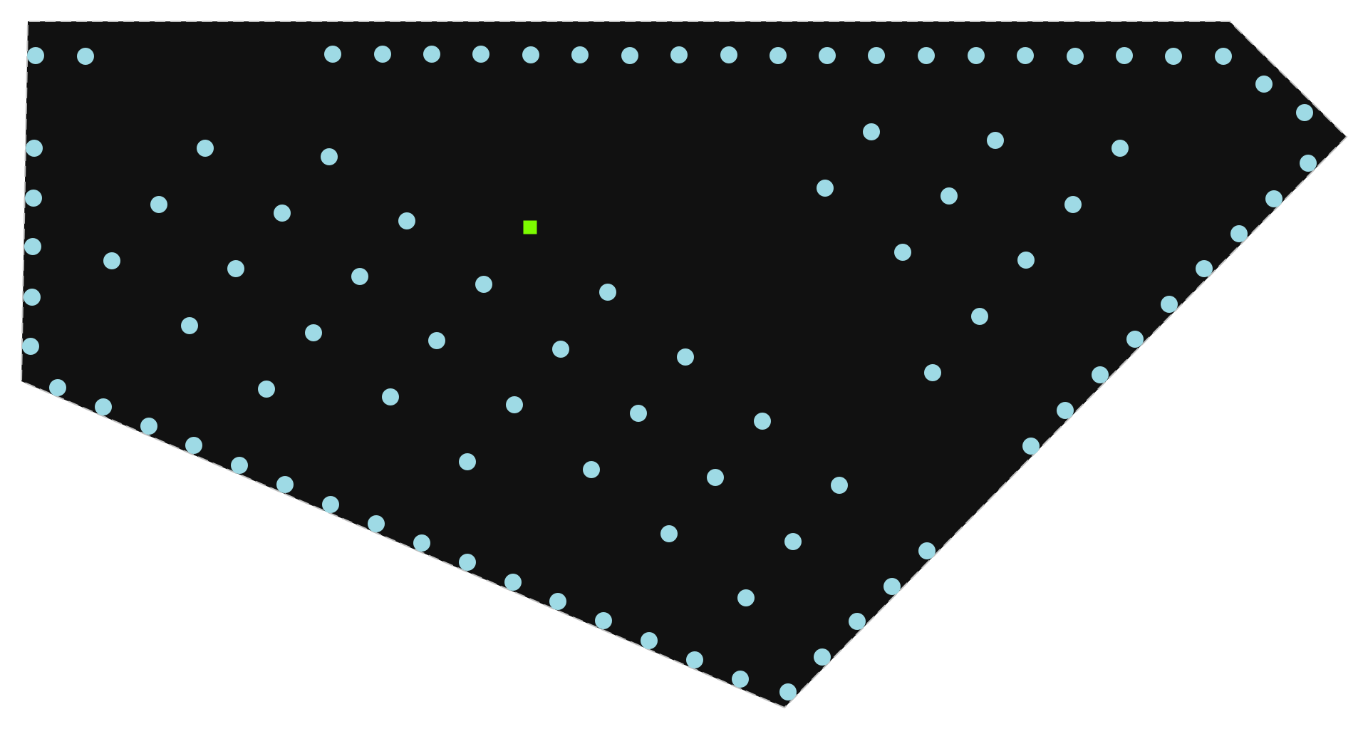
Plot the location to confirm that wfn contains the intended data.

Tip. In a notebook, put wfn as the last line of a cell to plot its current state.

• Before optimization (no G yet), it renders the location geometry L.

• If G exists (for example, after a call to optimize()), it automatically renders G.

Call wfn.plot_location() explicitly to plot only the location geometry. See 📊 Plotting for the available plotting methods.

wfn

2. Define a Router

Three built-in routers are available in OptiWindNet, one per optimization approach:

Router	Approach
EWRouter	constructive heuristic — sub-second
HGSRouter	meta-heuristic — configurable time budget
MILPRouter	exact optimization — reports an optimality gap

Their trade-offs are compared in Optimization approaches. See 📦 WindFarmNetwork for details about routers.

EWRouter

Create an EWRouter instance with no arguments to use its defaults. Every argument is optional.

from optiwindnet.api import EWRouter

ew_router = EWRouter()

HGSRouter

To use this router, create an instance of the HGSRouter class. The only required argument is time_limit, which defines how long the optimization is allowed to run (in seconds).

from optiwindnet.api import HGSRouter

hgs_router = HGSRouter(time_limit=1, seed=1234567)

MILPRouter

Create a MILPRouter instance with the following required arguments:

• solver_name: the MILP solver to use (e.g., 'ortools.cp_sat', 'gurobi', 'ortools.cbcbox')

• time_limit: maximum time allowed for solving (in seconds)

• mip_gap: acceptable optimality gap (e.g., 0.005 = 0.5%)

Optional arguments:

• verbose (default: False): set to True to display solver progress and detailed logs

• solver_options: dictionary of solver-specific parameters

• model_options: advanced model settings (e.g., topology, feeder configuration)

from optiwindnet.api import MILPRouter

milp_router = MILPRouter(
    solver_name='ortools.cp_sat',
    time_limit=20,
    mip_gap=0.005,
    solver_options={'random_seed': 1234567},
)

3. Run the optimization

EWRouter (sub-second)

%%timeit
res_ew = wfn.optimize(router=ew_router)

37.3 ms ± 478 μs per loop (mean ± std. dev. of 7 runs, 10 loops each)

wfn.solution_info()

{'router': 'EWRouter', 'capacity': 8, 'method': 'biased_EW', 'iterations': 84}

results.append(
    (
        wfn.solution_info()['router'],
        wfn.G.graph['topology'].value,
        f'{wfn.length():.1f}',
    )
)
results[-1]

('EWRouter', 'branched', '261192.1')

Plot the optimized network.

Note: Call wfn.plot() explicitly to plot the optimized network. See 📊 Plotting for the available plotting methods.

wfn

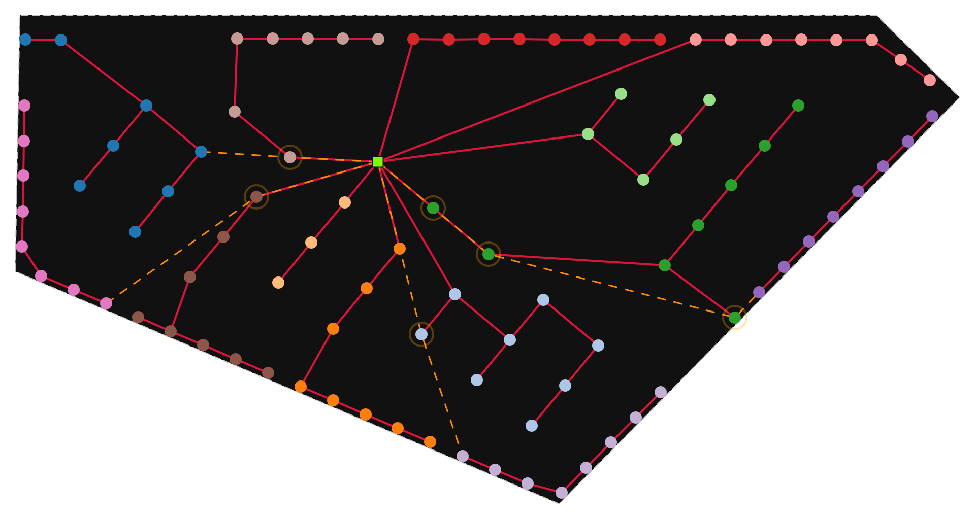
Note: Each call to .optimize() on the same WindFarmNetwork instance overwrites its stored solution and related information, including the network graph, cost, and length. Compare the updated length or plot with the preceding result to observe the replacement.

HGSRouter (fast — radial or ringed topology)

res_hgs = wfn.optimize(router=hgs_router)

wfn.solution_info()

{'router': 'HGSRouter',
 'capacity': 8,
 'solver_name': 'HGS-CVRP',
 'complete': False,
 'feeders_above_min': None,
 'feeders_exact': False,
 'balanced': False,
 'ringed': False,
 'repair': True,
 'max_retries': 10,
 'nbGranular': 20,
 'mu': 25,
 'lambda_': 40,
 'nbElite': 4,
 'nbClose': 5,
 'nbIterPenaltyManagement': 100,
 'targetFeasible': 0.2,
 'penaltyDecrease': 0.85,
 'penaltyIncrease': 1.2,
 'seed': 1234567,
 'nbIter': 20000,
 'nbIterTraces': 500,
 'timeLimit': 1,
 'useSwapStar': True,
 'runtime': 1.00029728}

results.append(
    (
        wfn.solution_info()['router'],
        wfn.G.graph['topology'].value,
        f'{wfn.length():.1f}',
    )
)
results[-1]

('HGSRouter', 'radial', '243214.0')

wfn

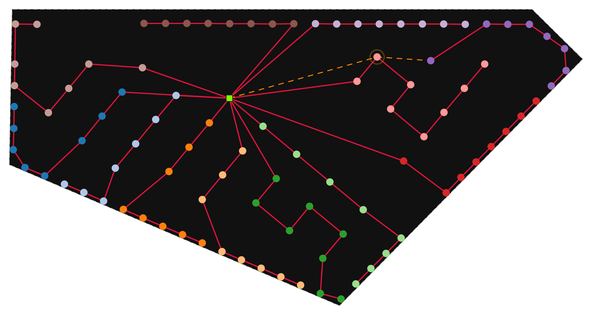
Note that the HGSRouter produces a radial or ringed topology, never a branched one. The three topologies are defined in Network topologies; the figure below contrasts them.

from IPython.display import HTML

from optiwindnet.api import ModelOptions
from optiwindnet.synthetic import toyfarm

wfn_toy = WindFarmNetwork(L=toyfarm(), cables=4)
opt_milp = {
    'mip_gap': 0.001,
    'time_limit': 5,
    'solver_name': 'ortools.cp_sat',
    'solver_options': {'random_seed': 1234567},
}

panels = []
for topology in ('radial', 'branched', 'ringed'):
    wfn_toy.optimize(
        router=MILPRouter(
            **opt_milp,
            model_options=ModelOptions(topology=topology, feeder_limit='minimum'),
        )
    )
    caption = f'<p style="color:#888">{topology.capitalize()}</p>'
    svg = wfn_toy.plot(infobox=False, tight=True).data
    panels.append(f'<div style="flex:1">{caption}{svg}</div>')

HTML(f'<div style="display:flex">{"".join(panels)}</div>')

Radial

Branched

Ringed

MILPRouter

MILP reports a bound and an optimality gap for its length model; routing detours can increase the delivered length. See Exact optimization.

Note:

• MILPRouter warm-starts by default: it reuses the solution already stored in the WindFarmNetwork, and builds one with a fast heuristic when there is none or the stored one does not fit the model — see Warm-starting.

• To solve cold instead, pass warmup=False; warmup_time is the budget for building a warm start.

• Set verbose=True to see warm-start messages in the logs.

res_milp = wfn.optimize(router=milp_router)

wfn.solution_info()

{'router': 'MILPRouter',
 'capacity': 8,
 'solver_name': 'ortools.cp_sat',
 'mip_gap': 0.005,
 'time_limit': 20,
 'topology': <Topology.BRANCHED: 'branched'>,
 'feeder_route': <FeederRoute.SEGMENTED: 'segmented'>,
 'feeder_limit': <FeederLimit.UNLIMITED: 'unlimited'>,
 'balanced': False,
 'runtime': 20.029517,
 'bound': 229556.31575552459,
 'objective': 240715.159901454,
 'relgap': 0.04635704768448201,
 'termination': 'FEASIBLE'}

results.append(
    (
        wfn.solution_info()['router'],
        wfn.G.graph['topology'].value,
        f'{wfn.length():.1f}',
    )
)
results[-1]

('MILPRouter', 'branched', '240866.2')

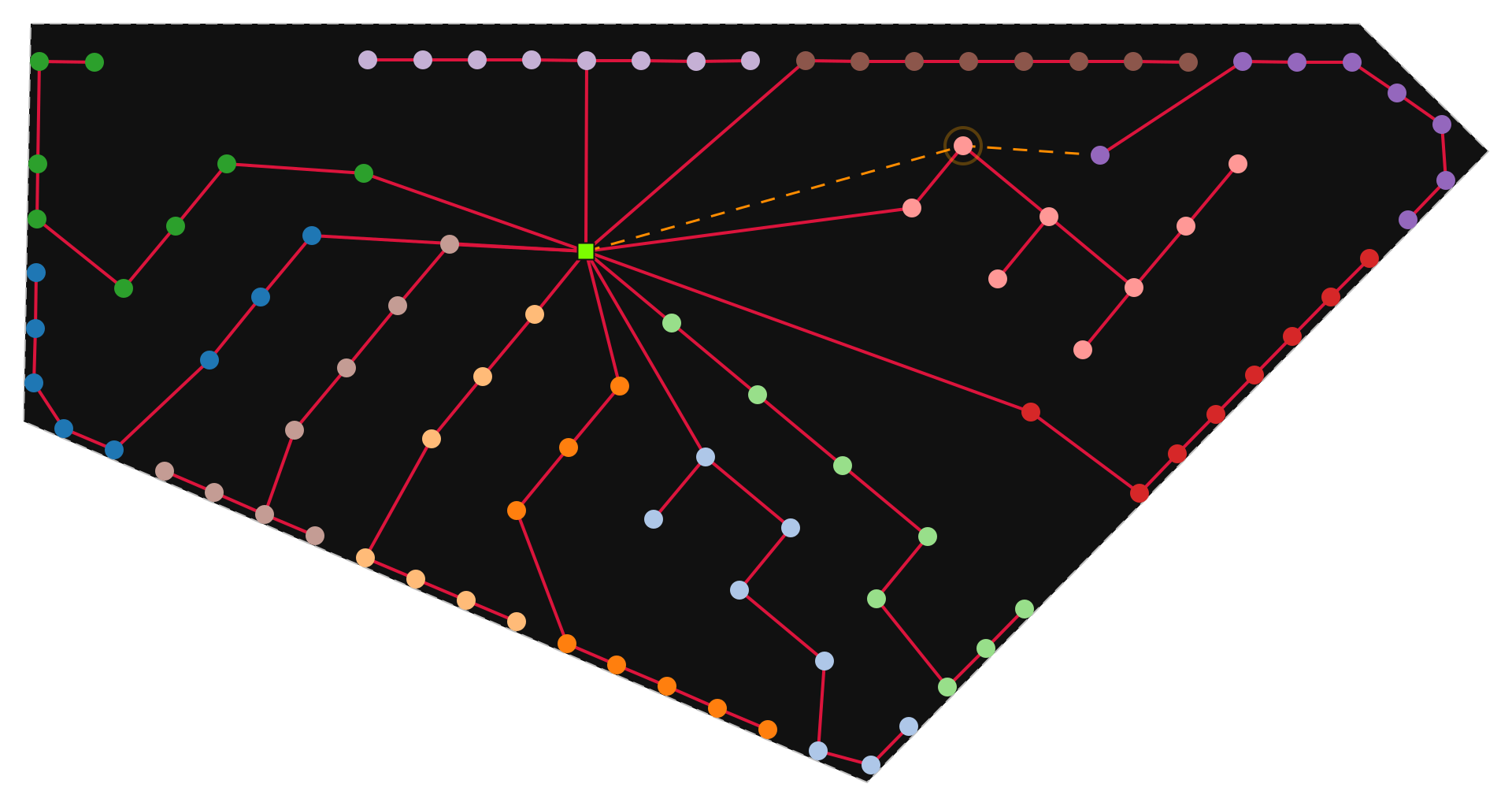
The two length values describe different stages of the solution. wfn.solution_info()['objective'] is the length optimized by the MILP on the available-links graph, before route reconstruction. wfn.length() sums the physical cable routes after PathFinder introduces any detours required by the navigation mesh. The routed length can therefore be slightly longer. Use objective to interpret the solver’s bound and relative gap, and wfn.length() for the final installed cable length. If cable prices are supplied, wfn.cost() reports the cost of the routed network. Length and cost often track each other, but the MILP gap is a guarantee about modeled length, not a bound on cost suboptimality. See Objective and reported cost.

wfn

Compare the results of the three routers:

from prettyTables import Table

Table(
    results,
    headers=('router', 'topology', 'length (m)'),
)

router	topology	length (m)
EWRouter	branched	261192.1
HGSRouter	radial	243214.0
MILPRouter	branched	240866.2